Miscellaneous Utilities

Nicholas Mikolajewicz

2020-05-28

Miscellaneous Functions

There are several additional functions that are worthwhile exploring in the XcalRep package.

Data import and prep

Prior to analysis, import data and preprocess as described in the Getting Started Vignette.

# import EFP and QC1 imaging phantom data
df.qc1 <-qc1
df.efp <- efp

# omit water-mimetic resin sections
df.qc1 <- dplyr::filter(df.qc1, section  != 1) # remove water mimic section 1
df.efp <- dplyr::filter(df.efp, section  != 4) # remove water mimic section 4
df.efp$section <- as.numeric(as.character(df.efp$section))
df.qc1$section <- as.numeric(as.character(df.qc1$section))

# combine datasets (ensure replicate sets aren't mixed)
df.qc1$replicateSet <- paste("q", df.qc1$replicateSet, sep = "")
df.efp$replicateSet <- paste("e", df.efp$replicateSet, sep = "")
all.data <- bind_rows(df.qc1, df.efp)


# create Calibration Object
co <- createCalibrationObject(all.data)

# get list of feature subsets to analyze
analyze.these <- analyzeWhich(co,
                              include.parameters = c("Tt.vBMD"))

# preprocess/filter data
co <- preprocessData(object = co,
                      analyze.which = analyze.these,
                      new.assay.name = "preprocessed.data",
                      which.assay = "input")

1) Mean-Variance Relationship: meanVarPlot

The mean.var.plot function enables users to explore the relationship between measurement means and variance, and may inform which precision error is more appropriate to report. The precision error measure that remains relatively constant across all values is preferred, as it does not misrepresent reproducibility for extreme values.

This relationship can be examined as either a scatter plot

meanVarPlot(co,
              which.data = "uncalibrated",
              which.plot = "scatter",
              which.parameter = "Tt.vBMD")

#> Warning in meanVarPlot(co, which.data = "uncalibrated", which.plot =
#> "scatter", : precision errors calculated based on replicateSet grouping

#> `geom_smooth()` using formula 'y ~ x'
#> `geom_smooth()` using formula 'y ~ x'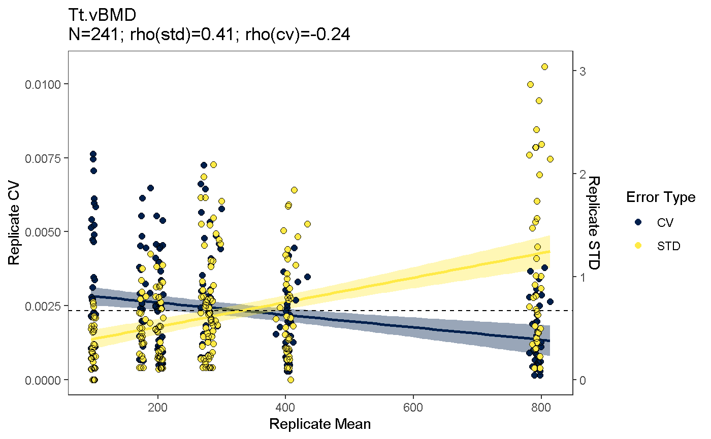

or boxplot

# requires troubleshooting
# error message: Error in eval(predvars, data, env) : object 'section' not found

# meanVarPlot(co, 
#               which.data = "uncalibrated", 
#               which.plot = "box", 
#               which.parameter = "Tt.vBMD")

2) Utility Functions:

cloneAssay If users i) create an analysis “checkpoint” to which they can return at a later time or ii) diverge in analysis pipelines for the current dataset, cloneAssay will duplicate the specified (or current) Assay within the current Calibration Object.

# duplicate current assay
co <- cloneAssay(co)

#> 
#> 'preprocessed.data' was successfully cloned

getAssay(co, which.assays = "all")

#> [1] "input"                  "preprocessed.data"      "preprocessed.data-copy"

deleteAssay A specified assay can be deleted using the deleteAssay function.

# duplicate current assay
co <- deleteAssay(co, which.assay = "preprocessed.data-copy")

#> 
#> 'preprocessed.data-copy' was successfully deleted.